Production Profiles
Decline curves, parent-child interference, associated gas from oil wells, and the unit economics of a shale gas well from spud to abandonment.
On the morning of Mon February 13, 2023, a production engineer in DeSoto Parish, Louisiana, opened the prior-day flow data on a Haynesville well that had reached total depth in May 2022, been fractured through 65 stages in late July, and been turned to flow through the gathering meter on Sun August 14, 2022. On day 30 the well averaged 28 million cubic feet per day. On day 90 it averaged 19. On day 180 it averaged 13. The print for Sun February 12, 2023 was 8.2 million cubic feet per day.
The decline was not anomalous. It was the well’s contract with the rock. The drilling and completion crews had done what they could do. From this point forward what mattered to the firm’s investors was not what the well produced this month, but the curvature of the line connecting today’s rate to the rate it would print three years and ten years out. Two wells with identical IP-30 rates can be worth twice as much as one another depending on how the line bends.
Modern shale economics live on that curve. The capital expenditure happens in the first year and is finished before the well has produced 30 percent of its eventual lifetime gas. The cash that pays back the well, and the cash that funds the next well on the same pad, comes from the long tail. A 10 percent operator discount rate compresses the tail but does not erase it. Whether the well returns capital depends on whether the curve a petroleum engineer fits in month four matches the cash the rock delivers in years two through fifteen.
Mitchell Energy’s vertical Barnett wells in the early 1990s produced for two to three years and stopped, and they would not fund a $10 million completion at any gas price. Cabot Oil and Gas’s early Susquehanna County Marcellus wells in 2008 to 2010 produced at high rates for years before they bent, and they repriced an entire basin. Production profile is the rock returning the capital. The capital does not get returned without the curve.
Flowback and the First 90 Days
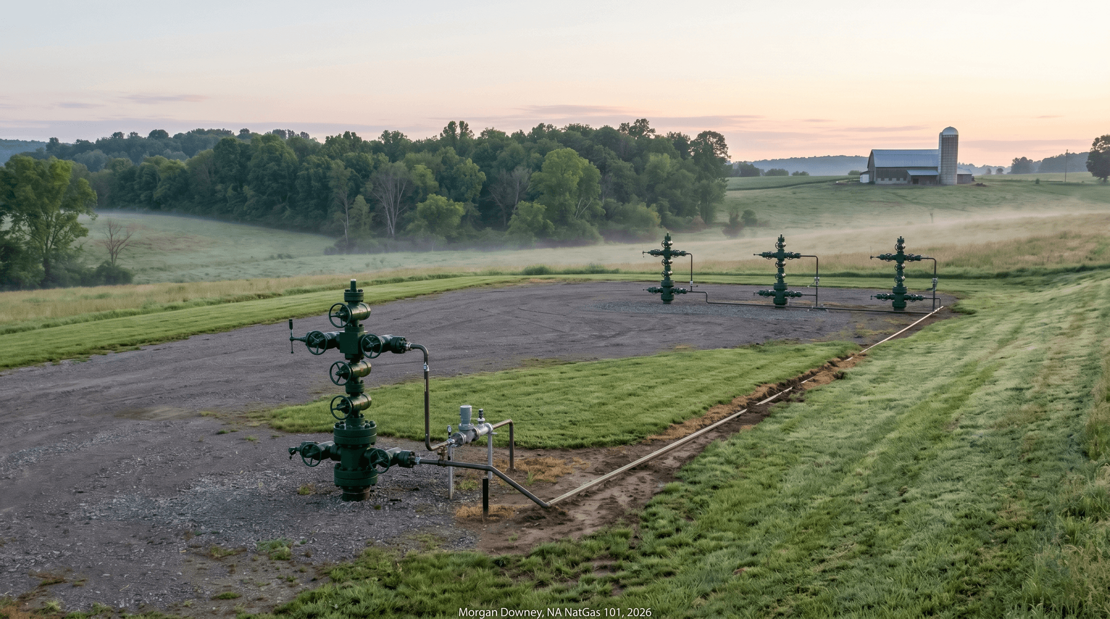
The completion crew finishes its drillout of the composite plugs, opens the wellhead to the flowback tank, and the well begins to flow back. The first fluid up the casing is the slickwater that went down. Within hours the choke at surface is being adjusted to manage the drawdown rate, the gas content of the returning fluid begins to climb, and the flowback specialist on the wellsite logs the rate, pressure, and chloride concentration of the produced fluid every two hours.
Choke management is the central operational decision of the first weeks. A wide-open choke maximizes early flowback rates and pulls the well rapidly toward peak gas production, but it can also damage the proppant pack at the perforations by accelerating fluid through the near-wellbore region faster than the rock can stabilize. Operators typically open the choke in stages of one-eighth or one-quarter inch at a time, watching the surface pressure response, the gas-to-water ratio, and the entrained-solids content of the flowback fluid. A standard Marcellus dry-gas choke schedule moves the well from a 12/64-inch initial setting to roughly 32/64 inch over the first 30 days, with operator-specific variations.
The chemistry of the flowback fluid evolves day by day. Total dissolved solids in the early flowback are dominated by the friction reducers and additives that went down with the slickwater, and chloride concentrations are low. Within two to three weeks, formation water begins to dominate the return stream and chloride concentrations climb sharply. By day 30 in a typical Marcellus completion, the produced fluid carries 60,000 to 150,000 milligrams per liter of dissolved chloride, against fresh-water levels around 50. The water company on the pad watches the chloride trajectory because it determines whether the fluid can be reused in a future completion or has to be sent to a saltwater disposal well.
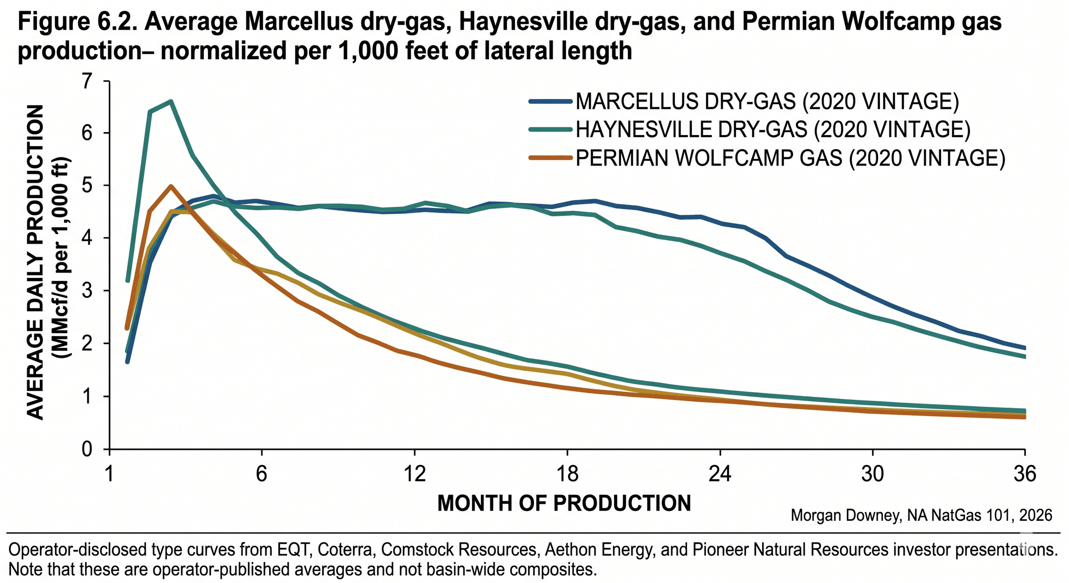
Gas production climbs as the water unloads. A typical Marcellus dry-gas well comes online at 4 to 8 million cubic feet per day in the first week and reaches a peak between day 30 and day 90, often above 20 million cubic feet per day at the highest-quality wells in the Susquehanna County core. Haynesville wells, drilled into deeper and higher-pressure rock, often peak earlier and at higher rates: 30 to 40 million cubic feet per day at the dry-gas core, and over 50 in the highest-IP wells.
The handoff from completion to production has a name. A well is turned in line, often shortened to TIL or TIL’ed in operator language, when the wellhead is opened to the gathering meter and gas first flows into the pipeline that carries it to a processing plant or interstate transmission point. Flowback into a tank battery on the pad is not TIL. The TIL date is the date of first sales gas across the gathering meter, the date the operator books the well into the producing inventory, and the date the meter starts the clock on the IP-30 calculation.
Operators report quarterly TIL counts as the leading indicator of operator-level production growth. EQT, Antero Resources, Coterra Energy, Range Resources, Comstock Resources, and Aethon Energy each disclose TILs by basin and target zone in their investor presentations. The TIL pace is watched as closely as rig count and DUC (drilled-uncompleted) inventory by equity analysts and supply modelers. A quarter with 30 Marcellus dry-gas TILs at the Susquehanna County type curve translates, after first-year decline, into a per-quarter incremental production layer that the Henry Hub market reads twelve to eighteen months later as the new well cohort rolls into the producing base.
The IP-30 metric, the average daily production rate over the first 30 days of flow, is the headline number operators report to investors and analysts use to benchmark wells against the type curve. IP-90 averages over 90 days and is more robust to a single high-flow day or an early choke transient. IP-180 captures the half-year arc and reflects whether the well’s plateau held. The metrics matter because reserves engineers fit decline curves through them and equity analysts back-cast type curves against them. They are also imperfect: a well with a high IP-30 and a steep early decline can produce less lifetime gas than a well with a lower IP-30 and a flatter curve, and operators who optimize completions only for IP-30 risk drilling wells that read well in the press release but underperform on capital return.
The operational handoff happens around the time the well reaches peak rate. The completions crew demobilizes its pumping spread and wireline trucks. The production team takes over the wellsite, with a reduced crew of one or two operators per pad and remote SCADA control of the choke and gathering valves from a central operations center. The well is now what the rock makes it.
Decline Curves: Hyperbolic, Exponential, Modified Hyperbolic
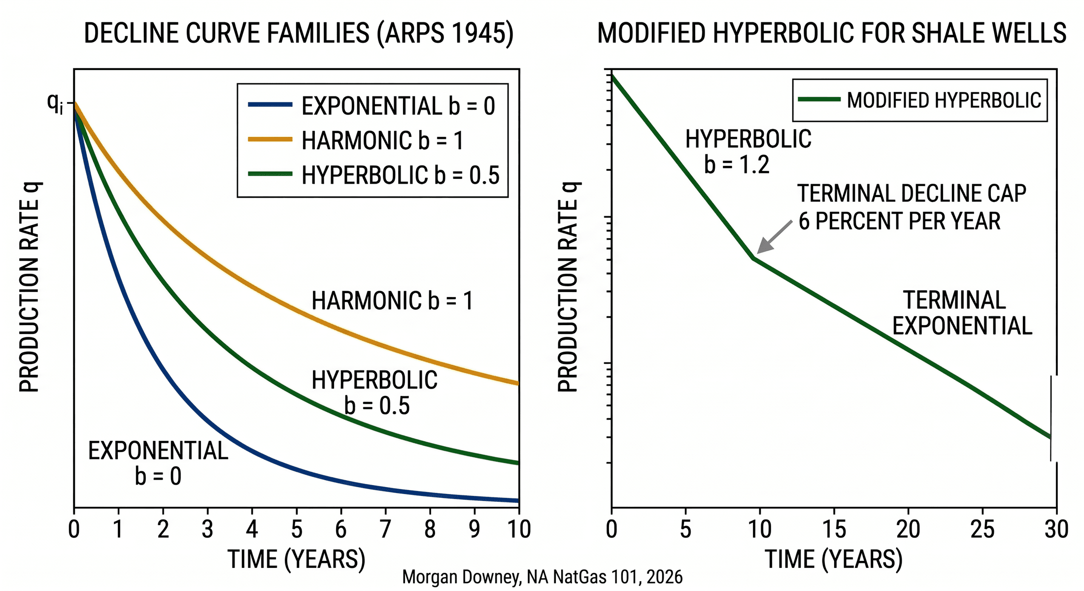
Petroleum engineers fit and forecast well production with the framework J.J. Arps published in "Analysis of Decline Curves" (Trans. AIME, Vol. 160, 1945). Arps’ framework defines three decline-curve families distinguished by the relationship between the rate of decline and the production rate.
Exponential decline is the special case where the decline rate is a constant fraction of the production rate per unit time. A well declining exponentially at 8 percent per month produces 92 percent of last month’s rate this month, regardless of the absolute level. Mathematically, q(t) equals q-sub-i times the exponential of negative D-sub-i times t, where q-sub-i is the initial rate, D-sub-i is the initial decline rate, and t is time. Conventional gas wells in mature fields, where reservoir pressure falls smoothly with cumulative production, fit exponential curves well.
Harmonic decline is the opposite extreme: the rate of decline falls inversely with cumulative production. A harmonically declining well decelerates as it ages, with the rate falling slowly enough that the cumulative production never converges to a finite value within engineering timeframes. Pure harmonic decline is rare in real producing wells but useful as a mathematical bound.
Hyperbolic decline is the general case. The rate of decline falls with cumulative production but more slowly than exponential and more quickly than harmonic. Arps parameterized the family with a b-factor between 0 and 1, where b equal to 0 recovers exponential decline and b equal to 1 recovers harmonic decline. The closed-form rate equation is:
q(t) = q_i / (1 + b * D_i * t) ^ (1/b)
Modern unconventional shale wells fit hyperbolic curves with b-factors typically between 0.8 and 1.5 in their early life. B-factors above 1.0 violate Arps’ original assumption that b lies in [0,1] and predict cumulative production diverging to infinity at long times, which is physically impossible. Reserves engineers handle the violation by capping the hyperbolic curve at a terminal exponential decline once the rate falls below a chosen threshold, typically 5 to 8 percent per year. The hyperbolic-then-exponential composite, called modified hyperbolic, is the standard decline-curve model for shale reserves work.
The rationale for high early-life b-factors in shale is geological. The well drains the stimulated reservoir volume around the wellbore first, then progressively pulls gas from rock farther into the matrix as pressure depletes near the fracture network. The transition from fracture-dominated flow to matrix-dominated flow stretches out the decline at long timeframes relative to a conventional reservoir, and the apparent b-factor in a fitted curve is high. The terminal-decline cap prevents the model from continuing the high-b extrapolation past the point where the physics breaks down.
The arithmetic of the cap matters for reserves valuation. A well producing at q-sub-i of 25 million cubic feet per day with a b of 1.4, an initial annual decline of 70 percent, and a terminal decline of 6 percent per year has very different cumulative production at year 30 from the same well with the same parameters but a terminal decline of 10 percent per year. The 4-percentage-point difference in terminal decline can change the calculated 30-year EUR by 10 to 20 percent. The choice of terminal decline is not a small number.
Decline-curve software is the working tool of the reserves engineer. PHDWin, Aries, and ARMR are the three packages most widely used in US oil and gas reserves work, with PHDWin (TRC Consultants) and Aries (Halliburton’s Landmark division) holding the largest market shares. The packages fit decline curves to historical production data, apply economic limits and price decks, calculate reserves under SEC and SPE-PRMS classifications, and produce the cash flow tables that anchor every internal valuation, every reserves report attached to a 10-K, and every reserve-based loan facility offered by a North American bank.
The Society of Petroleum Evaluation Engineers publishes guidance on shale reserves estimation that the SEC’s reserves disclosure framework defers to in practice. SPEE Monograph 3 (2010) and Monograph 4 (2016) establish the analytical methods and reasonable-certainty thresholds for booking proved, probable, and possible reserves on unconventional wells. Every reserves engineer running a Marcellus or Permian booking starts from those texts and works forward.
First-Year Decline and EUR
By the end of the first year, a modern shale well has lost 60 to 80 percent of its initial production rate. By the end of the second year, another 30 to 50 percent of what was left at the end of year one is gone. By year five, a typical well produces 5 to 15 percent of its IP-30 rate. By year ten, the rate is in single-digit percent of IP-30 and tracking the terminal exponential.
The arithmetic forces the economic structure of every shale program. A well that produces 30 percent of its EUR in the first 12 months and 50 percent of its EUR by month 24 is paid back, in present-value terms, on a calendar that depends almost entirely on the first-year cash flow. The capital is at risk for a short window. The remaining EUR pays for the next well’s drilling.
Estimated Ultimate Recovery (EUR) is the integral of the decline curve over the well’s producing life, truncated at 30 years of production or at the economic limit, whichever comes first. The economic limit is the production rate below which monthly operating costs exceed gross revenue at the assumed price deck. For a typical dry-gas Marcellus well producing at $3.00 per MMBtu Henry Hub flat, with $0.50 per Mcf operating cost net of basis, the economic limit is roughly 100 to 200 thousand cubic feet per day. Below that rate the well is shut in, recompleted, or refracked.
EUR per 1,000 feet of lateral, often shortened to EUR per foot when context is clear, is the standard normalization that lets engineers and analysts compare wells of different lateral lengths against the same yardstick. The numbers as of late 2024:
- Marcellus dry-gas core (Susquehanna and northern Wyoming counties, Pennsylvania): roughly 1.5 to 3.0 Bcf per 1,000 feet of lateral.
- Haynesville dry-gas core (DeSoto and Caddo parishes, Louisiana, and Harrison and Panola counties, Texas): roughly 2.0 to 3.5 Bcf per 1,000 feet.
- Permian Wolfcamp gas per 1,000 feet: depends sharply on the bench and the gas-to-oil ratio. Wolfcamp A in the Delaware sub-basin runs roughly 1.0 to 2.0 Bcf per 1,000 feet at typical GORs of 2,500 to 5,000 cubic feet per barrel. Lower-GOR Wolfcamp A wells in the Midland sub-basin produce less gas per foot but more oil.
EUR estimates are uncertain. The uncertainty compounds at long timeframes. A well with 18 months of production data fits hyperbolic parameters with reasonable confidence over the next two to three years, weak confidence at year five, and conjectural confidence at year 30. Reserves engineers handle the uncertainty by separating reserves into proved, probable, and possible categories and by applying conservative b-factor and terminal-decline assumptions on the proved bookings. Operator type-curve estimates of EUR routinely run 20 to 40 percent above the corresponding 1P (proved) reserves on the same wells, because the type curve uses the engineer’s central estimate while the proved booking uses the lower bound that the SEC reserves framework will accept.
The compounded uncertainty is why a 5-percentage-point shift in assumed terminal decline rate moves an entire reserves report’s value by hundreds of millions of dollars at scale, and why reserves auditors and SEC examiners spend disproportionate time on the terminal-decline assumption. The first 12 months of a well’s life are observed. The next 348 are forecast.
Type Curves vs Actual Well Performance
A type curve is the operator’s central estimate of what an average well in a given sub-area will produce over its life. Operators publish type curves to investors as the basis for drilling-inventory valuations, well-economics presentations, and capital-allocation arguments. A Marcellus operator pitching its dry-gas program to a reserves-based lender shows a type curve, the EUR underlying it, the implied 30-year cash flow at a stated price deck, and the well count to which that type curve applies across its acreage.
Type curves are constructed from a population of completed wells with similar geology and completion design. The operator selects a peer group of, say, 60 dry-gas wells turned to flow in the previous 18 months in a specific township-and-range cluster, normalizes each well to a common lateral length, and fits a single decline curve through the population. The resulting curve is the average. The standard deviation around the average is what the prospectus does not always show.
Actual wells distribute around the type curve with a wide spread. In a typical Permian sub-basin, the top decile of wells produces two to three times the median EUR, and the bottom decile produces 30 to 50 percent of the median. Marcellus dry-gas distributions are tighter than Permian distributions because the rock is more uniform across the core, but the spread between the best and worst wells in the same township still reaches a factor of three or four.
Three drivers explain the variance: rock quality, completion design, and operational execution. Rock quality varies even within a single township as thickness, total organic carbon, and clay content shift across short distances. Completion design varies by stage count, proppant intensity, fluid system, and cluster spacing, all of which are operator choices. Operational execution covers everything from how the wireline crew handled the perforations on stage 47 to whether the flowback choke was managed conservatively in week three. The combined effect of the three drivers produces a distribution whose width is large enough that the second-best well on a 12-well pad can outproduce the worst well by a factor of two.
Selection bias matters in operator marketing. The published type curve is the average across the historical peer group. The wells actually drilled in a given quarter cluster around the best acreage available, because operators allocate rigs to their highest-confidence locations first. A 2024 pitch to a reserves-based lender that anchors on a 2022 type curve from the same county will sometimes describe inventory that is qualitatively worse than the historical population. The reserves auditor’s job is to see through that and apply discounts to the lower-quality acreage in the inventory tail.
The opposite bias also runs. As completion design improves, recent wells outperform older type curves. A Marcellus dry-gas type curve fit to 2018 completions understates the EUR of a 2024 completion in the same township, because the 2024 completion runs longer laterals, higher proppant intensity, and tighter cluster spacing. Operators publish "current type curves" recalibrated each year to reflect the most recent completion designs, but the recalibration moves slowly enough that the published type curve always lags the rock by 12 to 24 months.
Tier 1, Tier 2, Tier 3 Acreage
Operators classify their leasehold by expected EUR per foot of lateral. The classification is informal and operator-specific but ubiquitous across investor disclosures. Tier 1 acreage is the rock that supports the operator’s published type curve, the locations where the rig goes first. Tier 2 acreage produces below the type curve, often 20 to 35 percent less per foot of lateral. Tier 3 acreage produces 40 to 60 percent below the type curve and is held mostly to satisfy lease-maintenance obligations rather than for active development. A typical Marcellus or Haynesville investor deck includes a remaining-locations slide that breaks the inventory into tiers: a 1,200-Tier-1 / 1,800-Tier-2 / 2,400-Tier-3 split, with implied years of drilling at the current pace, is the headline answer to “how long can the operator drill against the rock it controls.”
The economic gap between tiers is large. A Tier 2 location often carries a break-even gas price 20 to 50 percent above the Tier 1 break-even on the same capital expenditure, because the lower EUR has to pay for the same drilling and completion cost. A Tier 3 location frequently does not pay back at any plausible Henry Hub price and is drilled only when the operator has a held-by-production obligation that requires turning a well in line on that lease before the primary term expires.
The tier framework matters for portfolio valuation more than for any single well. The headline question on every shale operator’s investor day is how many years of Tier 1 inventory the company has left at the current rig pace. The answer is the bridge between current-quarter well economics and the long-term reinvestment story. EQT, Antero, Coterra, Range, and the other major Marcellus and Haynesville operators each disclose Tier 1 location counts by sub-basin and target zone, and equity analysts apply the operator-stated EUR per location and capex per location to model out a five-year-and-beyond cash flow trajectory. Permian operators do the same exercise across the Wolfcamp A, Wolfcamp B, Bone Spring, and Spraberry intervals, with tier classifications that span both depth and lateral position.
Tier classifications drift over time as completion technology improves. Acreage that EQT or Antero classified as Tier 2 in 2018 has been drilled at Tier 1 economics in 2024 because longer laterals, higher proppant intensity, and tighter cluster spacing have moved the type curve up. The reverse also runs: some Permian acreage classified as Tier 1 in 2014 has been quietly downgraded to Tier 2 after parent-child interference reduced the EUR available on infill locations. The framework is dynamic, not a one-time map, and the operator that publishes a static tier breakdown without recalibrating against recent completion results is signaling either confidence in stability or a marketing problem.
Parent-Child Interference and Well Spacing
Since 2018, the design of every Permian core completion has been shaped by parent-child interference. The mechanism is straightforward and the consequences are large.
When an operator drills an infill well between two existing producing wells, or beneath an existing well in a stacked-pay configuration, the new well’s frac propagates into rock whose pressure has been partially depleted by the existing wells. The infill well’s stimulated reservoir volume overlaps with the depleted reservoir volume around the parent. Three things follow. The infill’s frac fluid drains into the parent’s depleted reservoir rather than building pressure in the new wellbore’s drainage area. The parent well experiences a pressure response, often visible as a step change in flowing pressure within hours of the offset frac. The infill comes online at a lower IP and produces less lifetime gas than a comparable well drilled into virgin rock.
Pioneer Natural Resources, Concho Resources (acquired by ConocoPhillips in 2021), Diamondback Energy, and other Permian operators publicly discussed parent-child effects starting around 2017 and 2018 as the first generation of infill drilling tested the assumption that 660-foot lateral spacing inside the same bench could be replicated indefinitely. The reported child-well IP degradations against the unimpacted parent type curve ran 10 to 40 percent depending on operator, sub-basin, and time between parent completion and infill completion.
The industry response has been threefold. Well spacing has widened. At the 2017 peak of intensity, several Permian operators were running 660 feet between adjacent laterals in the same bench. By 2024 most operators had moved to 880 to 1,320 feet, with stacked-bench programs adding vertical separation through landing-zone diversification across the Wolfcamp A, Wolfcamp B, Bone Spring, and Spraberry intervals. Proppant intensity on infill wells has been reduced relative to the previous standard, because lower-intensity fracs propagate less far and reduce communication with depleted parents. Pre-fracking pressure-up operations have become standard practice. The parent is shut in for several weeks or months and water is injected up the parent’s wellbore to repressurize the depleted zone before the infill is fracked, restoring some of the parent’s contribution to the local stress field.
The economic effect of the design changes is non-trivial. Wider spacing reduces well count per section, which reduces inventory at the section level. Lower proppant intensity reduces the frac cost per well by 15 to 30 percent but also reduces the IP-30 of the infill. Pressure-up operations defer the infill drill schedule and consume produced water that otherwise would have gone to a disposal well or a recycled-fluid completion. Each of the three responses costs something. The combined costs are smaller than the EUR loss that uncontrolled parent-child interference would have produced if the 2017 spacing standard had been preserved.
The Permian core remains the basin where parent-child constraints bind hardest. The Marcellus dry-gas core also experiences parent-child effects but with less severity, because the dry-gas Marcellus has a single dominant producing interval and operators landed wells in well-separated rows on the original pad layouts rather than stacking and infilling within the same bench. The Haynesville sits between, with infill drilling becoming more common as the play matures and operators starting to encounter the same constraint that the Permian discovered six years earlier.
Associated Gas from Oil Wells
Most US natural gas does not come from gas-prone formations. Roughly 30 to 40 percent of US dry-gas production in 2024 came from wells whose primary target was oil, with gas as the associated co-product. The Permian, the Bakken, and the wet portions of the Eagle Ford produce gas as a function of oil output rather than gas price.
Gas-to-oil ratio (GOR) is the relevant measurement. GOR is the volume of gas produced per barrel of oil, expressed in cubic feet per barrel. It varies by basin, by formation, by sub-basin, and by the maturity stage of the producing well. The Permian Wolfcamp produces 1,500 to 5,000 cubic feet of gas per barrel of oil at the basin level, with sub-basin variation: the Delaware sub-basin’s gassier benches run higher GORs, the Midland sub-basin’s more oil-prone benches run lower. The Bakken in North Dakota produces roughly 1,000 to 2,500 cubic feet per barrel. The Eagle Ford runs a wider range depending on the thermal maturity window: black-oil wells in the deeper, hotter window produce 1,500 to 3,000, condensate wells produce 5,000 to 15,000, and the dry-gas wells in the deepest portions produce essentially no associated oil.
Associated gas is set by the oil rig count, not by the gas price. When WTI is at $80 a barrel, Permian operators continue running rigs, drilling oil-target wells, and producing whatever gas comes up the wellbore alongside the oil. When Henry Hub is at $1.80, the gas is sold for whatever the local hub will pay. When the local hub falls negative, the operator pays the pipeline to take the gas, or flares the gas under state regulation, or, if the regulator does not permit flaring, shuts in the well and loses the oil too.
The Waha hub in West Texas has traded at negative prices repeatedly since spring 2019, when growing Permian associated gas first outran pipeline takeaway capacity to the Gulf Coast and to the West Coast. Negative-pricing events recurred in 2020, 2022, and 2023 with multi-day stretches below zero and occasional single-day prints below negative $5 per MMBtu. New takeaway pipelines, including Whistler (commissioned 2021) and the Matterhorn Express (commissioned 2024), have eased the constraint without eliminating it.
The structural consequence is that Permian gas supply is largely insensitive to Henry Hub. A doubling of Henry Hub from $2 to $4 induces almost no incremental Permian gas drilling, because Permian capital is allocated against WTI economics and the gas comes up the wellbore regardless. A halving of WTI from $80 to $40 cuts Permian gas supply meaningfully, because the rig count falls. The Henry Hub price reflects the marginal supply cost of dry-gas-targeted production from the Marcellus and Haynesville. Permian gas is inframarginal in most price regimes.
Well Economics: Break-Even Price and NPV
The break-even gas price is the Henry Hub flat price at which the discounted future cash flows from a well exactly equal the upfront capital expenditure. The 10 percent operator discount rate is the standard convention for break-even disclosures, though some investors prefer 15 percent for risk-weighted comparisons and some operators publish PV-10 (proved reserves valued at a 10 percent discount) alongside PV-15. Net present value (NPV) at a given price is the sum of discounted future cash flows minus capex. A positive NPV at a stated price means the well returns capital plus the discount rate at that price; a zero NPV is the break-even.
The cash flow stack of a single shale well is:
- Gross gas revenue: production rate times the gas price at the wellhead, with basis discounts to local hubs (Dominion South or Tennessee Zone 4 for the Marcellus, Henry Hub for the Haynesville with a small basis, Waha for the Permian).
- Severance, ad-valorem, and federal income taxes.
- Royalty payments to the mineral owner: 12.5 to 25 percent of gross revenue.
- Lease operating expenses: $0.40 to $0.80 per Mcf in the Marcellus and Haynesville at typical 2024 cost structures, $0.70 to $1.20 per Mcf-equivalent in the Permian where water-handling costs dominate.
- Gathering, processing, and transportation (GP&T): $0.30 to $0.70 per Mcf in the Marcellus and Haynesville, with higher charges to firm-shipped paths to the Gulf Coast LNG load center.
Subtracting the cost stack from gross revenue produces a per-Mcf operating margin, which when multiplied by monthly production and discounted produces the present value of the well’s cash flow stream. The capex, drilling plus completion, is netted against the present value to produce NPV.
Break-even gas prices for modern wells, as of late 2024, by basin:
- Marcellus dry-gas core: roughly $1.50 to $2.00 per MMBtu Henry Hub flat.
- Haynesville dry-gas core: roughly $2.50 to $3.50 per MMBtu Henry Hub flat.
- Eagle Ford condensate window: roughly $2 oil-equivalent or lower, because the condensate liquid stream and the higher-value wet gas pay for the well at oil prices well below $50.
- Permian Wolfcamp: essentially insensitive to gas price. The oil revenue at $60 to $80 WTI repays the well multiple times before gas revenue contributes meaningfully.
The geography of US shale drilling activity follows the break-even ranking. The Marcellus dry-gas core has the lowest gas-price break-even and produces gas regardless of Henry Hub level above $2. The Permian produces gas as a function of WTI. The Haynesville is the marginal dry-gas basin, ramping up when Henry Hub is above $3 and slowing when Henry Hub falls below $2.50. The Henry Hub forward curve and the Permian rig count between them determine the gas supply that meets US demand and feeds the Gulf Coast LNG export terminals.
The arithmetic is simple. The capital expenditure is real money paid in year zero. The cash that returns it is forecast from a hyperbolic curve fit to 18 months of data. The price at which the discounted forecast equals the capital is the threshold below which operators stop drilling. When the gas market wants more supply, it pays the break-even price of the marginal play. When the gas market is oversupplied, the marginal play stops drilling and the supply curve adjusts.
Cabot’s Susquehanna Marcellus, 2008-2010
Cabot Oil and Gas was a Houston-based operator with leased acreage in the dry-gas portion of the Marcellus shale in northeast Pennsylvania when it drilled its earliest wells in Dimock and Springville townships, Susquehanna County, in 2008 and 2009. The first wells came online at IP-30 rates above 25 million cubic feet per day at a time when industry consensus held that a "good" Marcellus well would produce 4 to 6 million cubic feet per day at peak.
The economic implication was immediate. A well that comes online at five times the assumed rate produces three to four times the assumed EUR, not by virtue of a steeper curve but because the higher initial rate scales the entire forecast. The dry-gas Marcellus type curve that operators had carried into 2008 became obsolete on the wells Cabot drilled in 2009. The Pennsylvania producers extended their leasing programs north and east. Acreage that had traded at $200 per acre in 2007 traded at $5,000 in 2010 in the Susquehanna County core.
Cabot’s market capitalization roughly tripled between 2009 and 2014 on the production its Susquehanna County core acreage delivered. The company merged with Cimarex Energy in 2021 to form Coterra Energy. The original wells were still producing in 2024, sixteen years after they came online, on the long tail of decline curves that remained well above the 2008 industry assumption. The dry-gas Marcellus type curve those wells defined is the type curve every Susquehanna County operator still drills against.
The well produces gas. The next problem is moving the gas from the wellhead to the customer, and Chapter 9 turns to gathering, compression, dehydration, and processing.